Editor's note: Data type is an important concept in statistics. Machine learning and data science developer Niklas Donges gave a brief introduction to the different data types. Understanding these data types can help perform appropriate exploratory data analysis (EDA) on the data set-one of the most underrated parts of machine learning projects.
Introduction
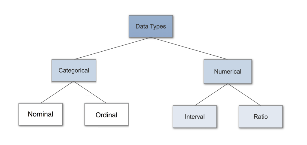
Understanding different data types is the key prerequisite knowledge required for Exploratory Data Analysis (EDA), and it also helps you choose the correct visualization method. You can think of data types as a way to categorize different types of variables. We will discuss the main variable types and corresponding examples. Sometimes we call it the measurement scale.
Category data
Categorical data represents characteristics, such as a person’s gender, language spoken, and so on. The category data can also use numerical values ​​(for example: 1 means female, 0 means male).
Nominal data
The nominal value refers to the qualitative discrete unit used to label variables. You can directly think of them as "tags". Note that the title data is out of order. Therefore, if you change the order of the name and value, its semantics will not change. Here are some examples of nomenclature features:
Gender: female, male.
Languages: English, French, German, Spanish.
The gender feature above is also called a "dichotomous" value because it contains only two categories.
Order data
Ordinal value refers to discrete, ordered qualitative units. In addition to being ordered, it is almost the same as the name data. For example, the educational background can be represented by the order value:
junior high school
High school
the University
Postgraduate
Note that the difference between junior high school and high school is not the same as the difference between high school and university. This is the main limitation of order data, and the difference between order values ​​is unknown. Therefore, the order value is usually used to measure non-numerical characteristics, such as pleasure and customer satisfaction.
Numerical data
Discrete data
Discrete data (discrete data) values ​​are different and scattered, in other words, can only accept some specific values. This type of data cannot be measured but can be counted. It is basically used to represent information that can be classified. For example, the number of times a coin is tossed heads up 100 times.
You can check whether you are dealing with discrete data through the following two questions: Can you count it? Can it be cut into smaller and smaller parts?
Conversely, if the data can be measured but not counted, it is continuous data.
Continuous data
Continuous data means measurement. For example, height.
Continuous data can be divided into interval data (interval data) and ratio data (ratio data).
Equidistant values ​​refer to ordered units with equal intervals, that is, equidistant variables contain ordered values, and we know the interval between these values. For example, using equidistant data to represent temperature:
-10
-5
0
+5
+10
+15
The problem with equidistant values ​​is that they have no "true zeros". Take the example above, 0 degrees is not absolute zero. In addition, we can add and subtract equidistant values, but cannot multiply and divide equidistant values ​​or calculate ratios. Because there is no "true zero", many methods of descriptive statistics or inferential statistics cannot be applied.
The equal ratio value has all the characteristics of the equal distance value, and it also has absolute zero. Therefore, not only can add and subtract, but also multiply and divide. Height, weight, length, absolute temperature, etc. are all equal ratios.
Why is the data type important?
Data type is a very important concept, because statistical methods can only be applied to specific data types. You need to analyze continuous data and categorical data in different ways. Therefore, understanding the type of data you are dealing with allows you to choose the correct analysis method.
Below we will revisit each of the data types mentioned above to understand what statistical methods they can apply. In order to understand some of the properties we will discuss, you need to have an understanding of descriptive statistics. If you are not familiar with this, you can read the introduction to descriptive statistics I wrote.
Statistical method
Nominal data
When processing nominal data, you collect information in the following ways:
Frequency The number of occurrences in a period of time or in the entire data set.
Ratio The frequency is divided by the sum of the frequencies of all events to get the ratio.
Percentage I don’t think this needs to be explained.
Mode The most frequent occurrence is the data with the highest frequency.
Visualization methods You can use pie charts or histograms to visualize nominal data.
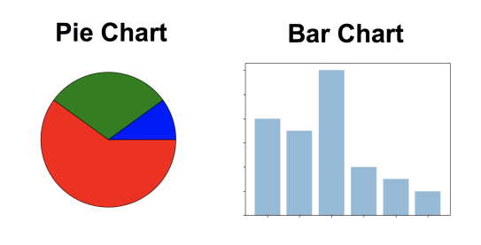
Left: Pie chart; Right: Histogram
Order data
When you are dealing with ordinal data, you can use the above method for nominal data, but in addition, you can also use some additional tools. In other words, you can use frequency, ratio, percentage, and mode to summarize ordinal data, and you can also use pie charts and histograms to visualize ordinal data. In addition, you can also use:
Percentile Calculate the cumulative percentile of sequential data from small to large. The data value corresponding to a certain percentile is called the percentile of this percentile. Percentiles can be used to describe discrete trends in data.
The median is the 50th percentile, which divides the data into equal upper and lower parts. The median can be used to describe the intermediate trend of the data. For example, if we use sequence data to represent the capacity of Starbucks coffee: medium cup, large cup, and extra large cup. Then, the median is the big cup (that is, the real middle cup is the big cup).
Interquartile range The difference between the 75th percentile and the 25th percentile is the interquartile range. The interquartile range provides a brief overview of the discrete trend of the data.
Continuous data
Most statistical methods can be used for continuous data. You can use percentile, median, interquartile range, mean, mode, standard deviation, interval.
You can visualize continuous data using rectangular or box plots. The intermediate trend, dispersion, shape and kurtosis of the distribution can be seen from the rectangular chart. Note that the histogram does not reflect discrete values, so we sometimes use box plots.
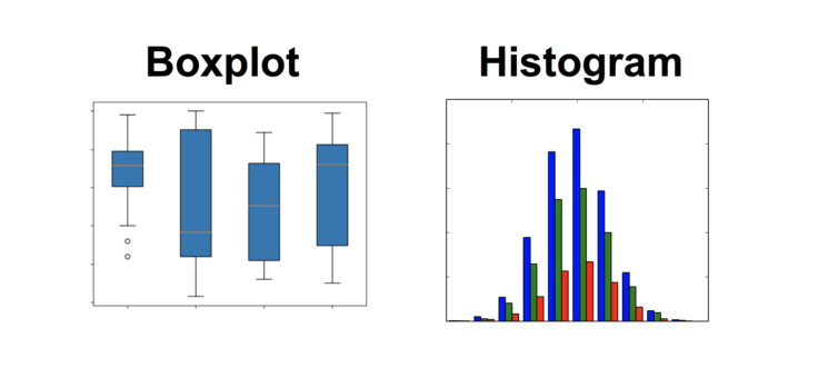
Left: box plot; right: rectangular plot
to sum up
This article discusses the different data types commonly used in statistics. You have understood the difference between discrete data and continuous data, and what is nominal data, sequence data, isometric data, and proportional data. In addition, you now know the statistical methods and visualization methods that can be applied to each data type. If you perform exploratory analysis on a given data set, you will find these very useful.
The latest Windows has multiple versions, including Basic, Home, and Ultimate. Windows has developed from a simple GUI to a typical operating system with its own file format and drivers, and has actually become the most user-friendly operating system. Windows has added the Multiple Desktops feature. This function allows users to use multiple desktop environments under the same operating system, that is, users can switch between different desktop environments according to their needs. It can be said that on the tablet platform, the Windows operating system has a good foundation.
Windows Tablet,New Windows Tablet,Tablet Windows
Jingjiang Gisen Technology Co.,Ltd , https://www.jsgisengroup.com