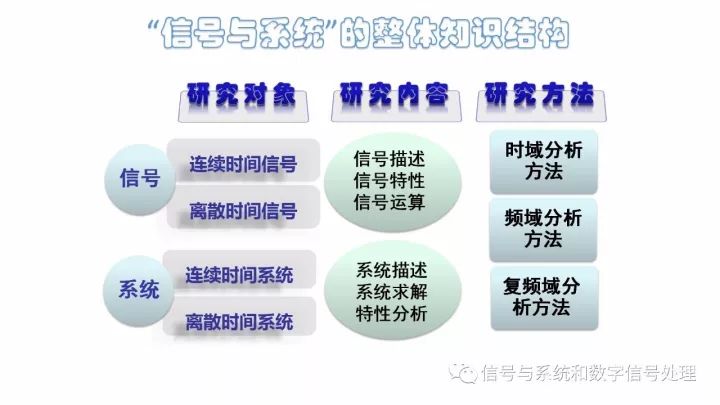
The "Signals and Systems" course content can be summarized as: two objects, three analysis methods, and three major transformations. Among them, two objects refer to signals (including continuous-time signals and discrete-time signals) and systems (including continuous-time systems and discrete-time systems); three analysis methods refer to time-domain analysis methods, frequency-domain analysis methods, and complex frequency domains. Analysis methods (the latter two are called transform domains); the three major transforms are the Fourier transform, the Laplace transform, and the Z transform.
We use these methods to study how to describe a signal, how to analyze the characteristics of the signal, how to operate on the signal, how to describe a system, how to solve the system's output (response), and how to analyze the system's characteristics. Learning these contents is the basis for future research on signal processing and system design.
The time domain analysis includes three parts: First, some basic concepts of signal and system; Second, the signal time domain analysis method; Third, the system time domain analysis method.
First, some basic concepts of signals and systems
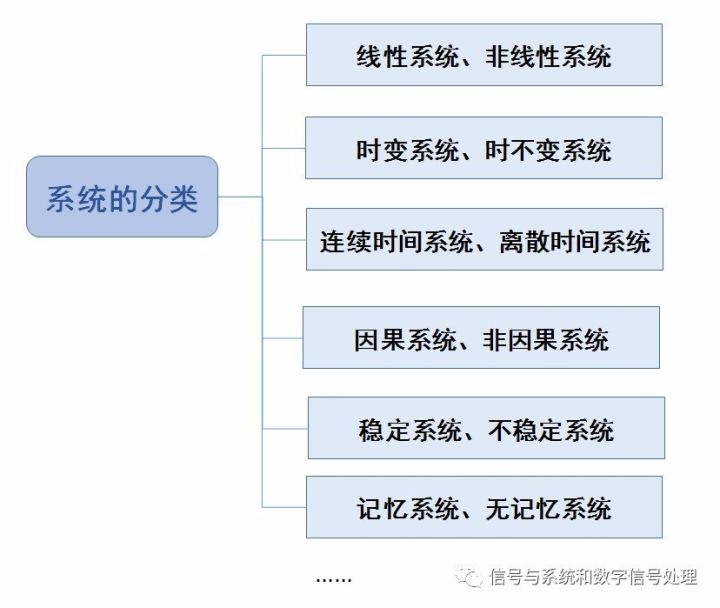
It includes two elements: signal and its description and classification, system and its description and classification. As shown in Figure 1 below.
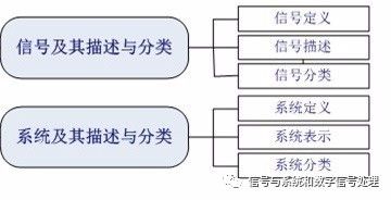
figure 1
Among them, "signal classification" and "system classification" are two key points.
In our course, signals are represented by "functions." Signals can be classified from different perspectives.
The signal classification includes:
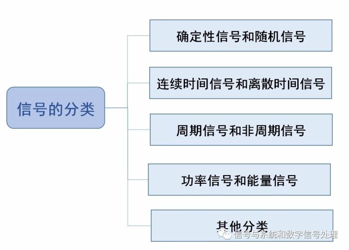
figure 2
Focus on two of them:
Continuous-time signals, discrete-time signals and analog signals, digital signals
The former focuses on whether the independent variable is continuous, while the latter focuses on whether the function value is continuous or not. In general, we refer to a signal in which both the argument and the function are continuous as an analog signal, and a signal in which both the argument and the function value are discrete are called digital signals.
Power signal, energy signal
This is a difficult point.
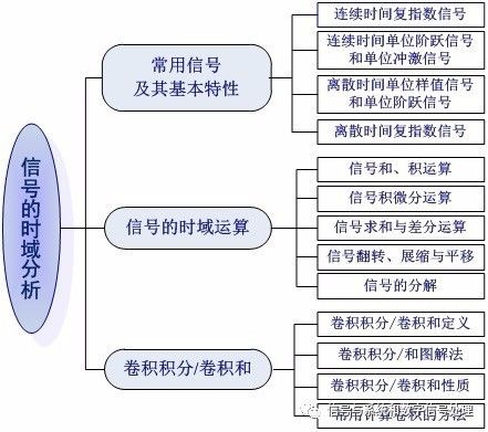
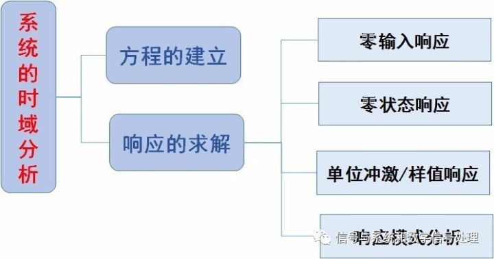
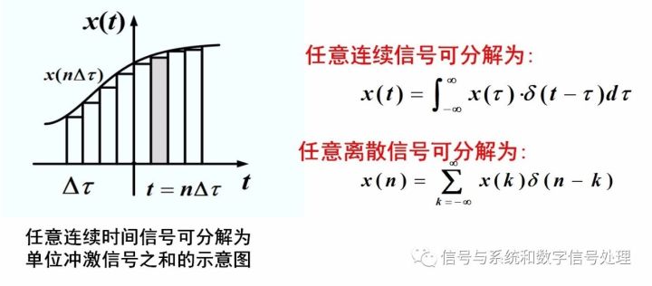
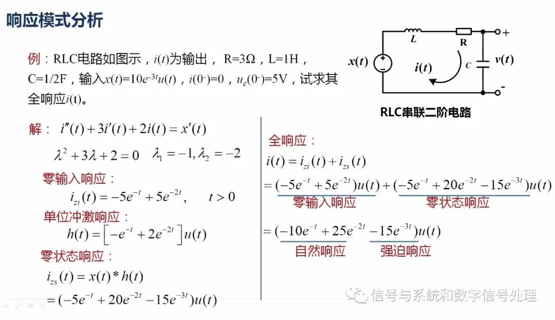
If the signal energy E satisfies: 0 If the signal's average power P satisfies: 0 Note: The two are mutually exclusive, that is, the average power of the energy signal must be zero; and the total energy of the power signal must be infinite. Most periodic signals are power signals, and non-periodic signals of limited duration are generally energy signals. Note that this is not absolute. The system's classification includes: image 3 There are two key points and difficulties: The determination of linear systems and nonlinear systems Time-varying system and time-invariant system These two contents were analyzed in detail in the previous article. See the determination of system linearity and time-invariance - one of the key difficulties in "Signals and Systems" Second, the signal time domain analysis method Time domain analysis of signals, including three contents, as shown below: Figure 4 (I) Common signals and their basic characteristics Focus and Difficulty: Unit Impulse Signals (B) Signal Time Domain Operations Focus and Difficulty: Signal Flipping, Zooming, and Panning (c) Convolution integral/convolution sum Focus and Difficulties: Definition, Properties, Calculation of Convolution Review suggestions: (1) Deeply understand the relationship between functions and signals This part of the content, related to the function of mathematics, to understand the physical meaning of the signal and its relationship with the function, with special attention to all kinds of signals have their corresponding physical model. (2) Note the relationship between signals The signals introduced in this chapter are many and can be divided into two types of signals after carding. One is a signal described by an ordinary function. The core is a complex exponential signal. It derives a DC signal, an actual exponential signal, an imaginary exponential signal, a sinusoidal signal, and the like. The second type is a signal described by a singular function, with emphasis on the impulse signal. It can generate impulse signals by differentiating it, some high-order derivative impulse signals, and integral can generate step signals and ramp signals. Third, the system time domain analysis method The time domain analysis of the system can be summarized as two big problems, as shown in the figure below. Figure 5 (a) The establishment of equations That is, a mathematical model is used to describe the system, a continuous-time system uses a differential equation, and a discrete-time system uses a difference equation. Our research object is the LTI (linear time invariant) system, so the equations describing the system are constant coefficient linear differential/difference equations. This part is not the focus. (B) Solution and Analysis of Response Includes four aspects: 1, zero input response 2. Unit impulse response h(t)/unit sample response h(n) 3, zero state response 4, response mode analysis Here are the following questions: First, the two major premises of time domain analysis: The first premise is that any signal can be decomposed into impulse signals (this part is not expanded, see Figure 2). In the second premise, the system discussed has a linear time-invariant system, so the system response can be decomposed into zero input responses. With the sum of the zero-state responses, the zero-state response can again be expressed as the sum of the impulse responses. In short, it is "the decomposition of signals, the synthesis of responses." Figure 6 Second, about zero time: Zero Hour: The time when the system was started, that is, the moment when the motivation was added. 0-Moment: Instant before the stimulus is added, 0+ Moment: Instant after the stimulus is added. 0-state: 0-time system state; 0+ state: 0+ time system state. The jump of the starting point - the transition from 0 - to 0 + state is a difficult problem. See Zheng Junli textbooks. Third, the solution to the response is the solution of the equation. The solution to the differential equations learned in high numbers (classical method): Full solution (full response) = homogeneous solution + special solution. Signal and System Lessons: Full response = zero input response + zero state response. What are the differences and connections between these two? Zero-input response, zero-state response: This is divided from the point of view of who is generating/causing this part of the response. Zero-input response is the input zero, the response generated by the system's initial energy storage; zero-state response is the system's initial energy storage is zero, the response generated by the external excitation. The homogeneous solution and special solution: It is divided from the perspective of who decides the form of the response mode. The form of the function of homogeneous solution is only related to the characteristics of the system itself. It is determined by the characteristic pattern of the system and is called the natural response of the system. The function form of the special solution is determined by the form of the external excitation signal and is called the forced response of the system. See the example shown below. Figure 7 Summarized as follows: Natural response = part of the zero input response + zero state response determined by the system characteristic root Forced response = part of the zero-state response that is determined by the input signal signature pattern in other words: Zero input response = part of natural response Zero-state response = Another partial natural response + forced response Fourth, unit impulse response / unit sample response Is a special zero-state response, where is it? The initial energy storage of the system is zero and only the response generated by the unit impulse signal. Solving method: continuous system, using impulse balance method; discrete system, using recursive method. Fifth, remind everyone that the time-domain solution method of the response is not important (the solution of the system response here can also be solved by the Laplace transform and z-transform methods). Interface Drivers Receivers Transceivers Shenzhen Kaixuanye Technology Co., Ltd. , https://www.iconlinekxys.com